The Canonical Equation of Adaptive Dynamics

What it means
The equation describes how the value of an ecological trait (z) evolves depending on the per capita mutation rate (μ), the variance of mutation effects (σ²), the population size at equilibrium (N^* ) and the selection gradient (the last factor). W(z', z) is called invasion fitness and is measured as the per capita growth rate of a morph with trait value z' in an environment where a morph with a trait value z dominates (the resident trait). Note that the derivative in the last factor, i.e. the slope of the invasion fitness, is taken with respect to the mutant trait z' and evaluated at the resident trait value z.

Implications and importance
The equation is derived for mutation-limited evolution in large, monomorphic, asexual populations (Dieckmann and Law 1996). Changes in the trait value are assumed to be small and occur as successful mutant populations establish and replace the resident population. It is biologically straightforward to see why the different factors in the equation affect the rate of evolution. To start with, the product of and N^* dictates how often mutations arise in the population. The factor 1/2 appears in the equation because under directional selection half of the mutations in a one-dimensional trait are bound to go in the 'wrong' direction. Higher variance in the mutation effects (σ;²) increases the rate of evolution by making the mutational steps longer. The slope of the invasion fitness around the resident trait value indicates how much fitness increases (or decreases) with a small mutational step. Evolution will be faster with a steeper slope since the likelihood of a successful invasion increases when the relative fitness advantage of the mutant over the resident is high. This slope also affects the direction of evolution such that z evolves towards higher values when the slope is positive and vice versa. Evolution will come to a halt when the slope of the invasion fitness is zero.

The canonical equation of adaptive dynamics, and generalisations of it, is especially useful for dealing with frequency-dependent selection and situations where the ecological feedback environment is affected by the evolutionary change. It has strong connections to evolutionary game theory and can for example be used to study gradual evolution to an Evolutionary Stable Strategy, ESS, or to evolutionary branching points (Geritz et al 1998, McGill and Brown 2007). Applications include food web evolution, speciation, fisheries management and the evolution of cooperation.

The canonical equation is related to other approaches to describe gradual evolution such as quantitative genetics or strategy dynamics. The approaches differ mainly in assumptions about the genetic variation (e.g. mutation-limited evolution vs. standing genetic variation) and whether or not ecological feedback is affecting evolution or not (changing vs. fixed adaptive landscape).

Jacob Johansson

Further reading:
Dieckmann U. and Law R. 1996. The dynamical theory of coevolution: A derivation from stochastic ecological processes. Journal of Mathematical Biology 34: 579–612

Geritz, S., É. Kisdi, E., G. Meszéna, G., and J. A. J. Metz, 1998. Evolutionarily singular strategies and the adaptive growth and branching of the evolutionary tree. Evolutionary Ecology 12: 35-57.

Champagnat, N., Ferrière, R., Ben Arous, G. (2001) The canonical equation of adaptive dynamics: a mathematical view. Selection 2, 73-83 .

Waxman, D. and Gavrilets, S. 2005. 20 Questions on Adaptive Dynamics. Journal of Evolutionary Biology 18: 1139-1154

McGill, B., and J. Brown. 2007. Evolutionary game theory and adaptive dynamics of continuous traits. Annual Review of Ecology, Evolution and Systematics 38: 403-435.

Species-Area relationship

S = cA^z

What it means
The equation states the relationship between an area (A) and the expected number of extant species (S) within that area. The constants c and z define the shape of the nonlinear relationship (Rosenzweig 2000). With an increasing area the expected number of species inhabiting that area is also increasing at a rate mainly dictated by z.

Where does it come from?
Originally the relationship, presented above, was theoretically derived from a species-abundance framework (Preston 1962). Given the assumption of a lognormal distribution of species abundances in a community, Preston derived the equation and calculated the z-value to be 0.27. This provided an empirically testable theory of biodiversity in island biogeography as well as mainland regions of different size.

Explanation and implications
The species-area relationship (mainly described by the exponent z above) can be explained by fundamental eco-evolutionary processes such as migration, speciation and extinctions which ultimately are driven by mechanisms such as niche availability, density dependence and species ranges (McGlade 1999). Although all mechanisms possibly are ubiquitous, some may be more important under certain conditions than others.. For example, large geographical areas include more diverse habitats, and hence more niches, facilitating high species diversity. In addition the degree of migration to and from the island, dictated by island area and isolation, has been identified as an important factor affecting the relationship.
In mainland areas with similar conditions the relationship can be explained by population size and geographical range of the species (McGlade 1999). As geographical area is decreased, population sizes and species ranges also decrease. This may give rise to an increase in extinction rate. Conversely, increasing population size and range facilitate speciation as large populations with large ranges often contain large genetic variation and are split into allopatry more often.

It has been shown that the coefficient c is often dependent on the taxon and biogeographical region, whereas z is more stable and has been estimated to fall between 0.20-0.35 for mainland biogeography and 0.12-0.17 for island biogeography (MacArthur 1969). These parameter estimations often fall below the theoretical value derived by Preston. Lower z-values than predicted can, for example, indicate high immigration of transient species from surrounding areas. Conversely, large z-values may indicate large islands or geographical areas which include several biomes whose species can evolve as independent assemblages. The species-area relationship has often been used in conservation biology (Krebs 1999), but not always without problems (see e.g., He & Hubbell 2011)

Mikael Pontarp

Further reading
He, F. & Hubbell, S.P. (2011) Species-area always overestimate extinction rate from habitat loss. Nature, 473

Krebs, C.J. (1999) Ecological methodology. Addison-Welsy Educational Publishers. Menlo Park

MacArthur, H.R & Wilson, E.O. (1968) The theory of island Biogeography. Princeton university press. Princeton

McGlade, J. (1999) Advanced ecological theory. Blackwell sience. London

Preston .F.W. (1962) The canonical distribution of commonness and rarity. Ecology, 43

Rosenzweig, M.L (2000) Species diversity in space and time. Cambridge University Press. Cambridge.

The Marginal Value Theorem

What it means:
The foraging in a patch (i) should be abandoned when the rate of energy acquisition in that patch (the left-hand side) equals the average intake rate including travelling time (the right-hand side, I^*). E is energy gain and h is time spent in the patch. The assumptions is that all the animal is doing is searching for and handling food.

Implications and importance:
The theorem is based on the fact that resource acquisition often has diminishing returns and that it pays to leave an activity before the patch is depleted if there are alternative patches to exploit. Charnov (1976) and Parker & Stuart (1976) were the first to formalize this idea in evolutionary ecology.
One example solution to the Marginal Value Theorem (MVT) is

where h_i^* is the optimal patch residence time in patch i, s_i is the resource level in patch i, s_a is the average resource level across patches, k is a parameter determining the initial slope of the gain function in a patch, and t_s is the average travelling time between any two patches in the environment (Lundberg & Åström 1990). If patches are close to each other so little time is spent travelling, patch residence time decreases. The same is true if the average patch (i.e., the environment) is resource rich (high s_a). The richer the focal patch (high s_i), the longer the patch residence time should be.
The MVT has made innumerable predictions for resource use in patchy environments (e.g., bees visiting flowers, browsers feeding on trees, mice exploiting seeds). Imagine yourself picking apples in an orchard or having one or many pork chops to eat when hungry. How many apples do you leave behind before changing trees if they are close and full of apples as opposed to the reverse?

Per Lundberg

Further reading:
Charnov, E. L. 1976. Optimal foraging, the marginal value theorem. Theor. Pop. Biol. 9: 129-136
Lundberg, P. & Åström, M. 1990. Functional response of optimally foraging herbivores. J. Theor. Biol. 144: 367-377.
Parker, G. A. & Stuart, R. A. 1976. Animal behaviour as a strategy optimizer: evolution of resource assessment strategies and optimal emigration thresholds. Am. Nat. 110: 1055-1076.
Stevens, D. W., Brown, J. S. & Ydenberg, R. C. (eds) 2007. Foraging. Chicago Univ. Press.

Exponential growth

What it means
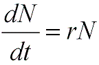
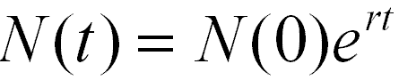
N is population density and t is time. This is the simplest model of population growth and assumes that the per capita growth rate, i.e., the difference between per capita birth and death rates, is a constant, r, often referred to as the intrinsic (per capita) growth rate. The solution of the differential equation above is

where N(0) is the population density at time zero. If r > 0 the population will grow to infinity, whereas if r < 0 it will decline towards zero.

Implications and importance
The 18th century reverend Thomas Malthus is often cited as the founder of the exponential growth model. This model is sometimes referred to as the exponential law (Turchin 2003); it certainly has similarities with the law of intertia in physics, and it is generally considered to be the first principle of population dynamics (e.g. Ginzburg 1986; Berryman 1999). Since it describes the dynamics of a population in a constant environment with no forces acting upon it, it efficiently serves as a starting point for more detailed models including e.g. structure (age, stage, space, etc), interactions and stochasticity. The stochastic version of the exponential growth model, which is a random walk on the log scale, is sometimes used in conservation biology for estimating extinction risks of populations at low density.


Further reading

Berryman, A. A. 1999. Principles of population dynamics and their applications. Stanley Thornes Publishers, Cheltenham, UK.

Ginzburg, L. R. 1986. The theory of population dynamics. I. Back to first principles. Journal of Theoretial Biology 122:385-399.

Turchin, P. 2003. Complex population dynamics. A theoretial/empirical synthesis. Princeton University Press, Princeton, NJ.

The Fear Equation

where μ is (perceived) predation risk, F is current fitness, and ∂F / ∂e is the marginal fitness gain from acquiring more energy from foraging.

What does it mean? Technically speaking, the equation represents the marginal rate of substitution of safety for food. It says that when the environment is risky (high rates of predation), when current fitness is high (e.g., if the animal is well fed), and when the marginal gain of more food is low, then one should be very risk averse, i.e., feel “fear”.

Where does it come from? It originates from Joel Brown’s seminal paper (Brown 1988) formulating the relationship between patch use, foraging rate and predation risk.

Importance: This idea has subsequently been much explored when studying foraging ecology, habitat selection, and the mechanisms of coexistence between competitors and predators and their prey. It elegantly shows how different fitness “currencies” (here, food and safety) can be translated into each other. This trick is often necessary when putting together reliable and realistic fitness functions for many problems in evolutionary ecology. It also determines the “landscape of fear” prey populations experience and it can be shown that this effect on the population can be greater than the actual killing of prey individuals. It also nicely explains the “Stalingrad effect”, i.e., the fearless behavior of the inhabitants of the city during the WWII battle under severe risk. They had with very low current “fitness” and extremely high marginal “fitness“ gain from some food. Think about similar situations yourselves!

Per Lundberg

Literature:

Brown, J.S. 1988. Patch use as an indicator of habitat preference, predation risk, and competition. Behav. Ecol. Sociobiol. 22: 37-47.

Brown, J. S. 1992. Patch use under predation risk: I. Models and predictions. Ann. Zool. Fennici 29:301-309.

Brown, J. S. & Kotler, B. P. 2004. Hazardous duty pay and the foraging cost of predation. Ecol. Lett. 7: 999-1014.

Fisher's Fundamental Theorem on Natural Selection

"The rate of increase in fitness of any organism at any time is equal to its genetic variance in fitness at that time." (Fisher 1930)

What it means

In brief, simplified terms, it means that natural selection will in all organisms tend to increase fitness. Evolution is in this simplified sense an optimizing process. Fitness, defined as per capita growth rate, is what is being optimized.

In more precise terms the statement needs a fair amount of qualification, almost word by word, to be as general as claimed. Fisher was by no means clear about the qualifications - they are mostly due to later interpretations (Price 1972).

”increase in fitness” - is the increase in the population mean additive genetic values of fitness. Further, it is the additive genetic values at the time of selection that counts.

”genetic variance” - the additive genetic variance, i.e. the variance in additive effects in the population.

Fitness can not increase forever, and Fisher was perfectly aware of it. However, natural selection will always tend to increase fitness while changes in the environment (such as an increased population density) can decrease fitness.

Edwards (1994) suggested a revised, modernized version of the theorem:
The rate of increase in the mean fitness of any organism at any time ascribable to natural selection acting through changes in gene frequencies is exactly equal to its genic variance in fitness at that time.

For further details see Price (1972) and Grafen (2003).

Implications and importance

The theorem is a key link between the mechanics of Mendelian genetics and evolution through natural selection, and thus a keystone of the modern evolutionary synthesis.

It has been viewed as a ’license’ for naturalists to think of organisms as optimizing agents, and pointing out exactly what is being optimized (Grafen 2003).  (Note: The process of evolution by natural selection is by no means dependent on genetics as we know it - evolution can work with many types of heritability. In this sense, organic life on Earth is but an example)

The theorem was for a long time disregarded as only applicable to special, simplified cases, but was later resurrected to its general status (Price 1972). This long delay can in most part be explained by the obscureness of Fisher’s writing and his unwillingness to express the theorem in more formal mathematics.

Further reading

Edwards, A. W. F. (1994) The fundamental theorem of natural selection. Biol. Rev. 69: 443-474

Fisher, R. A. (1930). The Genetical Theory of Natural Selection. Oxford, Oxford University Press.

Grafen, A. (2003). Fisher the evolutionary biologist. The Statistician 52(3): 319-329

Price, G. R. (1972) Fisher's "fundamental theorem" made clear. Ann. Hum. Genet., 36: 129-140