Exponential growth

What it means
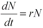
N is population density and t is time. This is the simplest model of population growth and assumes that the per capita growth rate, i.e., the difference between per capita birth and death rates, is a constant, r, often referred to as the intrinsic (per capita) growth rate. The solution of the differential equation above is

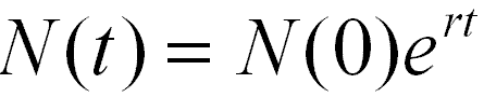
where N(0) is the population density at time zero. If r > 0 the population will grow to infinity, whereas if r < 0 it will decline towards zero.

Implications and importance
The 18th century reverend Thomas Malthus is often cited as the founder of the exponential growth model. This model is sometimes referred to as the exponential law (Turchin 2003); it certainly has similarities with the law of intertia in physics, and it is generally considered to be the first principle of population dynamics (e.g. Ginzburg 1986; Berryman 1999). Since it describes the dynamics of a population in a constant environment with no forces acting upon it, it efficiently serves as a starting point for more detailed models including e.g. structure (age, stage, space, etc), interactions and stochasticity. The stochastic version of the exponential growth model, which is a random walk on the log scale, is sometimes used in conservation biology for estimating extinction risks of populations at low density.


Further reading

Berryman, A. A. 1999. Principles of population dynamics and their applications. Stanley Thornes Publishers, Cheltenham, UK.

Ginzburg, L. R. 1986. The theory of population dynamics. I. Back to first principles. Journal of Theoretial Biology 122:385-399.

Turchin, P. 2003. Complex population dynamics. A theoretial/empirical synthesis. Princeton University Press, Princeton, NJ.

The Fear Equation

where μ is (perceived) predation risk, F is current fitness, and ∂F / ∂e is the marginal fitness gain from acquiring more energy from foraging.

What does it mean? Technically speaking, the equation represents the marginal rate of substitution of safety for food. It says that when the environment is risky (high rates of predation), when current fitness is high (e.g., if the animal is well fed), and when the marginal gain of more food is low, then one should be very risk averse, i.e., feel “fear”.

Where does it come from? It originates from Joel Brown’s seminal paper (Brown 1988) formulating the relationship between patch use, foraging rate and predation risk.

Importance: This idea has subsequently been much explored when studying foraging ecology, habitat selection, and the mechanisms of coexistence between competitors and predators and their prey. It elegantly shows how different fitness “currencies” (here, food and safety) can be translated into each other. This trick is often necessary when putting together reliable and realistic fitness functions for many problems in evolutionary ecology. It also determines the “landscape of fear” prey populations experience and it can be shown that this effect on the population can be greater than the actual killing of prey individuals. It also nicely explains the “Stalingrad effect”, i.e., the fearless behavior of the inhabitants of the city during the WWII battle under severe risk. They had with very low current “fitness” and extremely high marginal “fitness“ gain from some food. Think about similar situations yourselves!

Per Lundberg

Literature:

Brown, J.S. 1988. Patch use as an indicator of habitat preference, predation risk, and competition. Behav. Ecol. Sociobiol. 22: 37-47.

Brown, J. S. 1992. Patch use under predation risk: I. Models and predictions. Ann. Zool. Fennici 29:301-309.

Brown, J. S. & Kotler, B. P. 2004. Hazardous duty pay and the foraging cost of predation. Ecol. Lett. 7: 999-1014.

Fisher's Fundamental Theorem on Natural Selection

"The rate of increase in fitness of any organism at any time is equal to its genetic variance in fitness at that time." (Fisher 1930)

What it means

In brief, simplified terms, it means that natural selection will in all organisms tend to increase fitness. Evolution is in this simplified sense an optimizing process. Fitness, defined as per capita growth rate, is what is being optimized.

In more precise terms the statement needs a fair amount of qualification, almost word by word, to be as general as claimed. Fisher was by no means clear about the qualifications - they are mostly due to later interpretations (Price 1972).

”increase in fitness” - is the increase in the population mean additive genetic values of fitness. Further, it is the additive genetic values at the time of selection that counts.

”genetic variance” - the additive genetic variance, i.e. the variance in additive effects in the population.

Fitness can not increase forever, and Fisher was perfectly aware of it. However, natural selection will always tend to increase fitness while changes in the environment (such as an increased population density) can decrease fitness.

Edwards (1994) suggested a revised, modernized version of the theorem:
The rate of increase in the mean fitness of any organism at any time ascribable to natural selection acting through changes in gene frequencies is exactly equal to its genic variance in fitness at that time.

For further details see Price (1972) and Grafen (2003).

Implications and importance

The theorem is a key link between the mechanics of Mendelian genetics and evolution through natural selection, and thus a keystone of the modern evolutionary synthesis.

It has been viewed as a ’license’ for naturalists to think of organisms as optimizing agents, and pointing out exactly what is being optimized (Grafen 2003).  (Note: The process of evolution by natural selection is by no means dependent on genetics as we know it - evolution can work with many types of heritability. In this sense, organic life on Earth is but an example)

The theorem was for a long time disregarded as only applicable to special, simplified cases, but was later resurrected to its general status (Price 1972). This long delay can in most part be explained by the obscureness of Fisher’s writing and his unwillingness to express the theorem in more formal mathematics.

Further reading

Edwards, A. W. F. (1994) The fundamental theorem of natural selection. Biol. Rev. 69: 443-474

Fisher, R. A. (1930). The Genetical Theory of Natural Selection. Oxford, Oxford University Press.

Grafen, A. (2003). Fisher the evolutionary biologist. The Statistician 52(3): 319-329

Price, G. R. (1972) Fisher's "fundamental theorem" made clear. Ann. Hum. Genet., 36: 129-140